Engage NY Eureka Math Precalculus Module 5 Lesson 11 Answer Key
Eureka Math Precalculus Module 5 Lesson 11 Exploratory Challenge/Exercise Answer Key
Exploratory Challenge 1/Exercise 1
In this lesson, you will use empirical data to estimate probabilities associated with a discrete random variable and interpret probabilities in context.
Collect the responses to the following questions from your class:
Question 1: Estimate to the nearest whole number the number of hours per week you spend playing games on computers or game consoles.
Question 2: If you rank each of the following subjects in terms of your favorite (number 1), where would you put mathematics: 1, 2, 3, 4, 5, or 6?
English, foreign languages, mathematics, music, science, and social studies
Answer:
Responses may be displayed in raw form, tables, or graphs depending on the method you used to collect data from the class. The responses below are based on a class of 32 students.
Sample responses for Question 1 are given below.
Table: Number of Hours Playing Games on Computers or Consoles

Sample responses for Question 2 are given below.

Exploratory Challenge 1/Exercises 2–5: Computer Games
Exercise 2.
Create a dot plot of the data from Question 1 in the poll: the number of hours per week students in class spend playing computer or video games.
Answer:
Responses will vary. The plot below is based on the sample data given in Exercise 1.

Exercise 3.
Consider the chance experiment of selecting a student at random from the students at your school. You are interested in the number of hours per week a student spends playing games on computers or game consoles.
a. Identify possible values for the random variable number of hours spent playing games on computers or game consoles.
Answer:
Values include whole numbers from 1 to some number less than 24×7 = 168. (Records show that some teens actually do play games for two or three days straight, but this is unusual.)
b. Which do you think will be more likely: a randomly chosen student at your school will play games for less than 9 hours per week or for more than 15 hours per week? Explain your thinking.
ams:
Responses will vary.
Depending on the poll results students see displayed, if they think that their class is representative of students at the school, they may choose either option. Using the sample data above, students might suggest that chances seem more likely a randomly chosen student would play computer games less than 9 hours per week.
c. Assume that your class is representative of students at your school. Create an estimated probability distribution for the random variable number of hours per week a randomly selected student at your school spends playing games on computers or game consoles.
Answer:
The table below is a sample answer based on data given in Exercise 1.

d. Use the estimated probability distribution to check your answer to part (b).
Answer:
Responses will vary. A response based on sample data indicates that 0.31 of the class plays less than 9 hours per week, while 0.12 plays more than 15 hours of games on computers or game consoles.
Exercise 4.
Use the data your class collected to answer the following questions:
a. What is the expected value for the number of hours students at your school play video games on a computer or game console?
Answer:
Responses will vary. Based on the sample data, the expected value would be 9.7 hours.
b. Interpret the expected value you calculated in part (a).
Answer:
Responses will vary. If you were to randomly select a student and then randomly select a student again and do this many times finding the number of hours spent playing games, the average number of hours would be about 9.7 hours per week.
Exercise 5.
Again, assuming that the data from your class is representative of students at your school, comment on each of the following statements:
a. It would not be surprising to have 20 students in a random sample of 200 students from the school who do not play computer or console games.
Answer:
Responses will vary. Using the sample data, the estimated probability that students do not play any computer games is 0.09, which is about 18 of the 200 students. 20 is close to 18, so I would not be surprised.
b. It would be surprising to have 60 students in a random sample of 200 students from the school spend more than 10 hours per week playing computer or console games.
Answer:
Responses will vary. According to the sample data, the probability of playing more than 10 hours a week is 0.37, which would be about 74 students. 60 students is not too close to 74, but I do not think it is far enough away to be that unlikely, so I do not think it would be surprising.
c. It would be surprising if more than half of the students in a random sample of 200 students from the school played less than 9 hours of games per week.
Answer:
Responses will vary. Using the sample data, the estimated probability that students play less than 9 hours of computer games per week is 0.31, which is about 62 students. Half of 200 is 100, so I would be surprised if 100 of the students played less than 9 hours of games per week.
Exploratory Challenge 2/Exercises 6–10: Favorite Subject
Exercise 6.
Create a dot plot of your responses to Question 2 in the poll.
Answer:
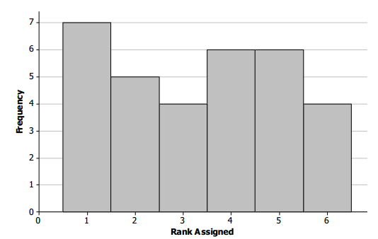
Responses will vary. Based on the sample data, the plot for Question 2 would be the following:

a. Describe the distribution of rank assigned.
Answer:
Responses will vary. For the sample data, the distribution of the ranks is fairly uniform, with not that much difference in the frequency with which each of the ranks was chosen.
b. Do you think it is more likely that a randomly selected student in your class would rank mathematics high (1 or 2) or that he would rank it low (5 or 6)? Explain your reasoning.
Answer:
Responses will vary. Using the counts in the sample data, students might observe that 12 people ranked math as 1 or 2, while only 10 people ranked math as a 5 or 6. So, two more people ranked it high than did low.
Exercise 7.
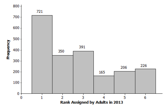
The graph displays the results of a 2013 poll taken by a polling company of a large random sample of 2, 059 adults 18 and older responding to Question 2 about ranking mathematics.

a. Describe the distribution of the rank assigned to mathematics for this poll.
Answer:
Responses will vary.
The distribution is skewed right with more people ranking mathematics with a 1 or 2 than with a 5 or 6.
b. Do you think the proportion of students who would rank mathematics 1 is greater than the proportion of adults who would rank mathematics 1? Explain your reasoning.
Answer:
Responses will vary. If students think that their class is representative of students in general, they may calculate the proportions or percentage and say more adults ranked it 1 than the students in their class. They may also ignore the data and respond with their beliefs.
Exercise 8.
Consider the chance experiment of randomly selecting an adult and asking her what rank she would assign to mathematics. The variable of interest is the rank assigned to mathematics.
a. What are possible values of the random variable?
Answer:
The values are 1, 2, 3, 4, 5, and 6.
b. Using the data from the large random sample of adults, create an estimated probability distribution for the rank assigned to mathematics by adults in 2013.
Answer:
Table: Rank Assigned to Mathematics (Adults in 2013)

c. Assuming that the students in your class are representative of students in general, use the data from your class to create an estimated probability distribution for the rank assigned to mathematics by students.
Answer:
Responses will vary. Sample response based on data from Question 2:
Table: Rank Assigned to Mathematics (Based on Sample Class Data for Question 2)

Note: Values may not add up to exactly 1 due to rounding.
Exercise 9.
Use the two estimated probability distributions from Exercise 8 to answer the following questions:
a. Do the results support your answer to Exercise 7, part (b)? Why or why not?
Answer:
Responses will vary. The probability distributions indicate that adults rank mathematics as 1 with a probability of 0.35, while students do so with a probability of 0.22.
b. Compare the probability distributions for the rank assigned to mathematics for adults and students.
Answer:
Responses will vary. Using the sample data, some students might note that the probabilities for ranking mathematics 6 and last for adults and for students were not that far apart. Others might note that for adults, the probabilities are quite large for a rank of 1 and then decrease with a little fluctuation. The probabilities for students are all about the same for all of the ranks.
c. Do adults or students have a greater probability of ranking mathematics in the middle (either a 3 or 4)?
Answer:
Responses will vary. Using the sample data, the estimated probability that a randomly chosen adult will rank mathematics as a 3 or 4 is 0.27 and that a randomly chosen student will rank it as a 3 or 4 is 0.32. These probabilities are not that far apart, so it does not seem that the two groups are that different.
Exercise 10.
Use the probability distributions from Exercise 8 to answer the following questions:
a. Find the expected value for the estimated probability distribution of rank assigned by adults in 2013.
Answer:
The expected value is 2.74.
b. Interpret the expected value calculated in part (a).
Answer:
Responses will vary. Given that the sample of 2, 059 people was random, if you asked lots of adults how they would rank mathematics, in the long run, the average ranking would be 2.74.
c. How does the expected value for the rank students assign to mathematics compare to the expected value for the rank assigned by adults?
Answer:
Responses will vary. Using the sample data, the expected value for students is 3.42, which indicates that students ranked mathematics lower than adults.
Eureka Math Precalculus Module 5 Lesson 11 Problem Set Answer Key
Question 1.
The results of a 1989 poll in which each person in a random sample of adults ranked mathematics as a favorite subject are in the table below. The poll was given in the same city as the poll in Exercise 6.
Table: Rank Assigned to Mathematics by Adults in 1989

a. Create an estimated probability distribution for the random variable that is the rank assigned to mathematics.
Answer:

b. An article about the poll reported, “Americans have a bit of a love-hate relationship with mathematics.” Do the results support this statement? Why or why not?
Answer:
Responses will vary.
Some students might note that the probability of ranks 1 and 2 is 0.43, and the probability of ranks 5 and 6 is 0.44. So, the probability that a randomly chosen adult from this city liked mathematics was almost the same as the probability that he did not like mathematics. Others might point out the probability that a randomly chosen person ranked math first was 0.24 and last was 0.27, which are only 0.03 apart, so the probability that the person loves math was about the same as the probability that he hates math.
c. How is the estimated probability distribution of the rank assigned to mathematics by adults in 1989 different from the estimated probability distribution for adults in 2013?
Table: Rank Assigned to Mathematics by Adults in 2013

Answer:
Responses will vary.
Students might say that the probability of ranking mathematics first was greater in 2013 or that the probabilities of ranking mathematics first and third in 2013 were greater than in 1989. The probability of ranking mathematics sixth in 2013 was less than half of the probability of ranking it sixth in 1989. The expected value in 2013 was a rank of 2.74, and in 1989 the expected value was lower with a rank of 3.56.
Question 2.
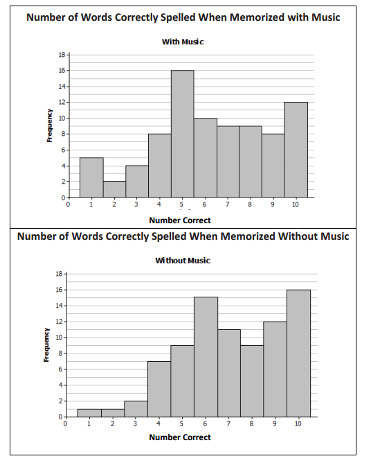
A researcher investigated whether listening to music made a difference in people’s ability to memorize the spelling of words. A random sample of 83 people memorized the spelling of 10 words with music playing, and then they were tested to see how many of the words they could spell. These people then memorized 10 different words without music playing and were tested again. The results are given in the two displays below.

a. What do you observe from comparing the two distributions?
Answer:
Responses will vary.
Some may observe that the people in the sample seemed to memorize more words without music than with music.
b. Identify the variable of interest. What are possible values it could take on?
Answer:
The random variable is the number of words spelled correctly. Possible values are integers 0 to 10.
c. Assume that the group of people who participated in this study are representative of adults in general. Create a table of the estimated probability distributions for the number of words spelled correctly when memorized with music and the number of words spelled correctly when memorized without music. What are the advantages and disadvantages of using a table? A graph?
Answer:
Responses will vary.
With music:

Without music:

Students might suggest the advantages of using a table are that you can see the actual probabilities, and the advantages of using a graph are that you can see the pattern or trend. It is almost easier to see that more words were spelled correctly when they were memorized without music from the graph because you can see the distribution seems to be more skewed left than the one for the number of words memorized with music.
A disadvantage of using a table might be that the differences in the probabilities are not always easy to sort out quickly; a disadvantage of using the graph is that you almost have to estimate the probabilities because you cannot see the actual values. (Note that some interactive technology will show the values if the cursor is dragged over the bar or point.)
d. Compare the probability that a randomly chosen person who memorized words with music will be able to correctly spell at least eight of the words to the probability for a randomly chosen person who memorized words without music.
Answer:
Responses will vary.
Students should compare the two probabilities: P(W ≥ 8 with music) = 0.35, while P(W≥8 without music) = 0.44. There is a 0.9 difference in the probability the person will be able to correctly spell at least eight words for the two conditions (music and no music).
e. Make a conjecture about which of the two estimated probability distributions will have the largest expected value. Check your conjecture by finding the expected values. Explain what each expected value means in terms of memorizing with and without music.
Answer:
The expected value for the number of words spelled correctly when memorizing with music is 6.27 words; without music it is 6.99 words. Assuming that the group of people who participated in this study are representative of adults in general, if you gave people lots and lots of lists of 10 words to memorize with and without music, over the long run, with music they would be able to spell 6.27 words and without music 6.99 words. The difference does not seem to be very large.
Question 3.
A random variable takes on the values 0, 2, 5, and 10. The table below shows a frequency distribution based on observing values of the random variable and the estimated probability distribution for the random variable based on the observed values. Fill in the missing cells in the table.
Table: Distribution of Observed Values of a Random Variable

Answer:
The missing cell in the Probability row has to be 0.03 because the sum of the probabilities has to be 1. The missing cell in the Frequency row has to be 28 because \(\frac{18}{32+x}\) = 0.3, \(\frac{12}{32+x}\) = 0.2, and \(\frac{2}{32+x}\) = 0.03, and solving for x in any of the equations yields x = 28.
Eureka Math Precalculus Module 5 Lesson 11 Exit Ticket Answer Key
The table shows the number of hours, to the nearest half hour per day, that teens spend texting according to a random sample of 870 teenagers aged 13–18 in a large urban city.
Table: Number of Hours Teenagers Spend Texting per Day

Question 1.
What random variable is of interest here? What are the possible values for the random variable?
ans;
The variable of interest is the number of hours to the nearest half hour teens spend texting per day. Possible values are 0, 0.5, 1, 1.5, 2, 2.5, 3, 3.5, 4, 4.5, and 5.
Question 2.
Create an estimated probability distribution for the time teens spend texting.
Answer:

*The total does not equal 1.00 due to rounding.
Question 3.
What is the estimated probability that teens spend less than an hour per day texting?
Answer:
0.29
Question 4.
Would you be surprised if the average texting time for a smaller random sample of teens in the same city was three hours? Why or why not?
Answer:
Responses will vary. Sample response:
I would be surprised because the expected value is 1.36 hours, and three hours is much larger than the expected value.