Engage NY Eureka Math Algebra 1 Module 2 Lesson 17 Answer Key
Eureka Math Algebra 1 Module 2 Lesson 17 Example Answer Key
Example 1.
Predicting the Pattern in the Residual Plot
Suppose you are given a scatter plot and least squares line that looks like this:
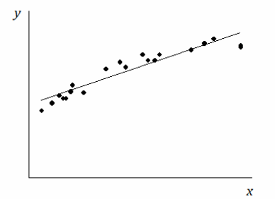
Describe what you think the residual plot would look like.
If students struggle, have them look carefully at the scatter plot. Point out that moving from left to right, the points initially tend to be below the least squares line, then move above it, and then below it. The residuals are negative, then positive, and then negative again. This means that the points in the residual plot will be below the horizontal axis, then above it, and then below it again.
The residual plot has an arch shape like this:
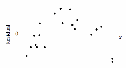
Why is looking at the pattern in the residual plot important?
Discuss with students that the residual plot provides another indication of the type of relationship between two variables.
Example 2.
The Meaning of Residuals
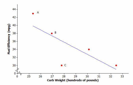
Suppose that you have a scatter plot and that you have drawn the least squares line on your plot. Remember that the residual for a point in the scatter plot is the vertical distance of that point from the least squares line.
In the previous lesson, you looked at a scatter plot showing how fuel efficiency was related to curb weight for five compact cars. The scatter plot and least squares line are shown below.
Consider the following questions:
→ What kind of residual does Point A have?
Answer:
Point A has a large positive residual.
→ What kind of residual does Point B have?
Answer:
Point B has a small positive residual.
→ What kind of residual does Point C have?
Answer:
Point C has a very large negative residual.
You also looked at the residual plot for this data set:
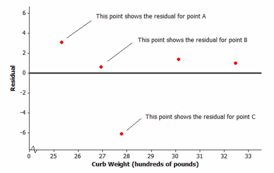
Your teacher will now show how to use a graphing calculator or graphing program to construct a scatter plot and a residual plot. Consider the following example.
Example 3:
Using a Graphing Calculator to Construct a Residual Plot
In an earlier lesson, you looked at a data set giving the shoe lengths and heights of 12 adult women. This data set is shown in the table below.
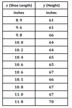
Use a calculator to construct the scatter plot (with least squares line) and the residual plot for this data set.
Calculation of the equation of the least squares line:
- From the home screen, go to the statistics editor by pressing STAT, ENTER.
- Enter the x-values into L1 and the y-values into L2.
- Press 2nd, QUIT to return to the home screen.
- Press STAT, select CALC, select LinReg(a+bx), and press ENTER.
- Type L1, L2, Y1 so that your entry reads LinReg(a+bx) L1, L2, Y1. (Y1 is accessed by pressing VARS and selecting Y-VARS, Function, 1.) Press ENTER.
- The y-intercept, a, and the slope, b, of the least squares line are displayed on the screen. (Also, the calculator stores in its memory a list called RESID, which is used in constructing the residual plot. Furthermore, since Y1 was included in the entry, the equation of the least squares line is entered as the Y1 equation in the Y = menu.)
Construction of scatter plot:
- From the home screen press 2nd, STAT PLOT.
- Select Plot1, and press ENTER.
- Select On. Under Type choose the first (scatter plot) icon, for Xlist enter L1, for Ylist enter L2, and under Mark choose the first (square) symbol.
- Press 2nd, QUIT to return to the home screen.
- Press Y =.
- Go to any unwanted graph equations and press CLEAR. Make sure that only Plot1 is selected (not Plot2 or Plot3).
- Press Zoom, select ZoomStat (option 9), and press ENTER.
- The scatter plot and the least squares line are displayed.
Construction of residual plot:
- From the home screen, press 2nd, STATPLOT.
- Select Plot2, and press ENTER.
- Select On. Under Type, choose the first (scatter plot) icon, for Xlist enter L1, for Ylist enter RESID, and under Mark choose the first (square) symbol. (RESID is accessed by pressing 2nd, LIST, selecting NAMES, scrolling down to RESID and pressing ENTER.)
- Press 2nd, QUIT to return to the home screen.
- Press Y =.
- First, deselect the equation of the least squares line in Y1 by going to the = sign for Y1 and pressing ENTER. Then deselect Plot1, and make sure that Plot2 is selected.
- Press Zoom, select ZoomStat (option 9), and press ENTER.
- The residual plot is displayed.
Note that when constructing a residual plot, you need the correct set of residuals to form the list called RESID. This is only the case if you have run the LinReg(a+bx) or LinReg(ax+b) command for the data set on which you are working.
Students often ask why we use LinReg(a+bx) rather than LinReg(ax+b). Explain how the two forms offer different representations of a linear equation. The more common convention in statistics is that a is the y-intercept and b is the slope, not vice-versa.
To save time and help students do the problem set, it might be worthwhile to give each student a copy of the calculator instructions.
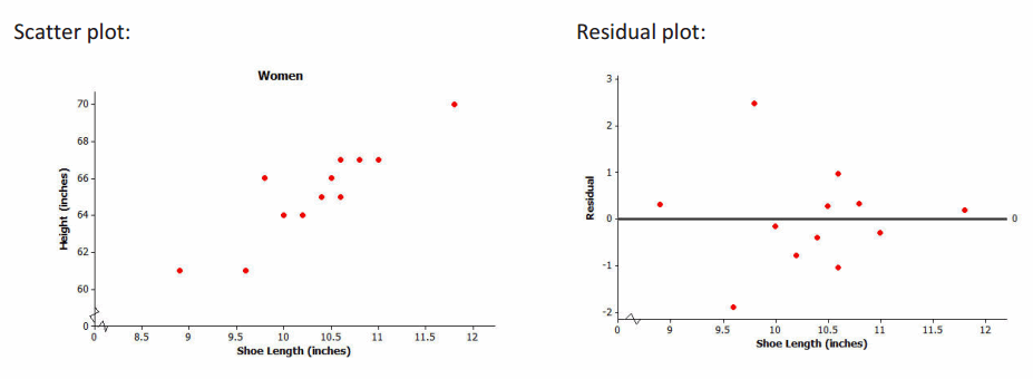
The equation of the least squares line for this example is y=32.679+3.1469x, where x is the shoe length (in inches), and y is the height (in inches). The scatter plot and residual plot are shown below.
Eureka Math Algebra 1 Module 2 Lesson 17 Problem Set Answer Key
Assist those students still needing help with the calculator or statistical program. If students are using a TI graphing calculator (e.g., a TI-83 or TI-84), tell them to turn off the STAT plot for 2. The first question asks only about the least squares line and the scatter plot.
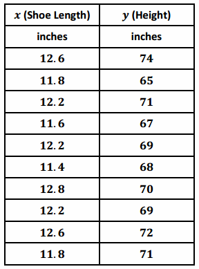
Consider again a data set giving the shoe lengths and heights of 10 adult men. This data set is shown in the table below.
Question 1.
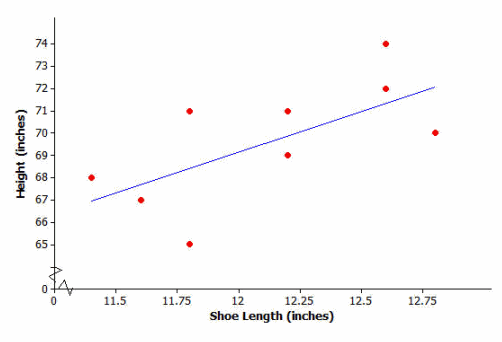
Use your calculator or graphing program to construct the scatter plot of this data set. Include the least squares line on your graph. Explain what the slope of the least squares line indicates about shoe length and height.
Answer:
The slope indicates that as the shoe length increases, so does the height. The following illustrates the scatter plot and residual plot from a calculator. (Note: If it is not possible for you to observe your students’ work on their calculators, have them show you a sketch of each graph.)
Question 2.
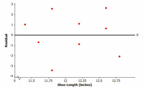
Use your calculator to construct the residual plot for this data set.
Answer:
See plot below.
Question 3.
Make a sketch of the residual plot on the axes given below. Does the scatter of points in the residual plot indicate a linear relationship in the original data set? Explain your answer.
Answer:
There is no curved pattern in the residual plot, and the points in the residual plot appear to be scattered at random around the zero line. This indicates that the relationship in the original data set is linear.
Eureka Math Algebra 1 Module 2 Lesson 17 Exit Ticket Answer Key
Question 1.
If you see a random scatter of points in the residual plot, what does this say about the original data set?
Answer:
A random scatter of points in the residual plot tells us that a linear function is an appropriate model for the relationship between the two variables in the original data set.
Question 2.
Suppose a scatter plot of bivariate numerical data shows a linear pattern. Describe what you think the residual plot would look like. Explain why you think this.
Answer:
Because the relationship between the two variables is linear, the residual plot would have a random pattern.